Querying is a useful tool for analyzing and editing specific parts of a map. After the Query command is clicked, the query is performed by selecting objects to include in the query, writing a query string to evaluate the objects, and selecting what action is performed to the objects returned by the query string. The Query Data command works similarly to the Query command, but the query is performed on the linked data. The Query Range command queries objects based on a specified distance from a single selected object. Since the Query Data command uses linked data, the Query Data command only works with boundary objects: polygons, polylines, and points. The Query and Query Range command can query all objects except text objects: boundary objects, rectangles, rounded rectangles, squares, ellipses, and circles.
This tutorial will show an example of each type of query command. First, open the HatchMap.gsm MapViewer sample file. The HatchMap.gsm file is a hatch map of the population of France by region.
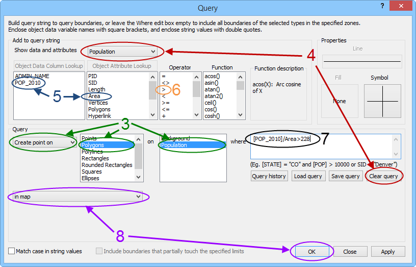
First, we will perform queries on the plot with the Query command. If you haven't done so already, open the HatchMap.gsm sample file. The numbers on the image below correspond to steps 3 - 8 in the Tutorial.
1. Click
the Analysis
| Query | Query command  .
The Add to query string (top)
section of the Query dialog is
used to create query strings and select properties to apply to queried
objects. The Query (bottom) section
of the Query dialog is read from
left to right, top to bottom as a sentence and defines the query. The
sentence takes the following form: Do
this to object(s)
on layer(s) where
query string 1 in
selection on layer(s) where query string 2.
.
The Add to query string (top)
section of the Query dialog is
used to create query strings and select properties to apply to queried
objects. The Query (bottom) section
of the Query dialog is read from
left to right, top to bottom as a sentence and defines the query. The
sentence takes the following form: Do
this to object(s)
on layer(s) where
query string 1 in
selection on layer(s) where query string 2.
2. First, we will create points on the regions where the population density is greater than 228 people per square mile. 228.05 is the median population density. The Object Property report, Transform command, and Statistics command were used to determine the median population density for the regions, so 11 points should be created. The Query section should read as, "Create point on Polygons on Population where [POP_2010] / Area > 228," when we are finished.
3. In the Query section, select Create point on from the first list. In the object list, click on Polygons, and in the layer (on) list, click Population. Clicking on a deselected object/layer selects it, and clicking on a selected object/layer deselects it.
4. If there is a query string in the where field, click the Clear query button. Next, make sure Population is selected in the Show data and attributes on list near the top of the Query dialog.
5. In the Object Data Column field, double-click on POP_2010. Notice that [POP_2010] is added to the where field. Next double click the divisor operator, /, in the Operator field. Finally, double click Area in the Object Attribute field.
Note: When the query string pulls data from a linked data column, the data column name must be surrounded by brackets. When text is used in the query string, it is surrounded by double quotes. Attributes and number values are not surrounded by special characters. More complex mathematical functions can be added to query strings with the Function field, but the query string does not have to contain a mathematical function.
6. Double-click the greater than operator, >, in the Operator field. Notice the operator is added to the query string in the where field.
7. Type "228" in the where field after the greater than operator. The final query string should be [POP_2010] / Area > 228.
8. In the in list, select in map, and click OK.
Now there should be 11 points on the map, indicating the regions with population densities greater than 228 people per square mile. Next, we will change properties for the points in regions with fewer than two million people.
1. First, let's move the points to another layer. Click the first point listed in the Object Manager, hold the SHIFT key, and click the last point listed in the Object Manager. Now that all 11 points are selected, click the Home | Clipboard | Move to Another Layer command. Select [New Layer] in the Move to Layer dialog, and click OK.
2 Click the Analysis | Query | Query command again. Now we will set up the query to apply properties to points within specific polygons. Select Apply properties to in the Query list. Select Points in the objects list. Select Layer #1 in the layer list, and click the Clear query button. The where field is left blank because the points referenced by it have no attributes or linked data to query.
3. Now, in the in field, select in polygons, and in the second layer list, select Hatch. Select Hatch in the Show data and attributes on list at the top of the Query dialog.
4. Next, type [POP_2010] < 2000000 in the lower where field. You can also use the Object Data Column and Operator lists to create the query string.
5. Click the Symbol button in the top right section of the Query dialog to open the Symbol Properties dialog. Click on the selection in the Symbol field to open the symbol palette and click on the filled diamond symbol (Symbol 6). Click OK in the Symbol dialog.
6. Click OK in the Query dialog.
Now the map includes three points for regions with populations under 2,000,000 people and a population density greater than 228 people per square mile, and eight points for the remaining regions with population densities greater than 228 people per square mile.
It is important to understand how the query lists, object and layer selections, and separate where fields function. The first line in the Query dialog was applying properties to points on Layer #1. If the points had attributes or linked data, we could have further defined the point selection by adding a query string to the first where field. The second line of the Query dialog was refining the query to include only points on Layer #1 that were contained within polygons on the Population layer with populations of less than two million people. Query strings, object and layer selections, and the in field selection must be made correctly to get the desired results.
Fortunately, many things can be queried different ways to get the same results. For example, the map resulting from the steps above could be recreated by performing the following two queries: "Create point on Polygons in Population where [POP_2010] / Area > 228 AND [POP_2010] < 2000000 in map" with Symbol 6 selected, and "Create point on Polygons in Population where [POP_2010] / Area > 228 AND [POP_2010] > 2000000 in map" with Symbol 0 selected. Notice with these queries, we wouldn't create another layer for the points or use the in polygons selection.
The Query Data command generates queries on linked data. In the following example, we will create a report for the four regions closest to the median value.
1. Click
the Analysis | Query
| Data command  to open the Query
Map Data dialog. Like the Query
command, the query is phrased like a sentence: "Do
this with # of objects
closest to value/object."
to open the Query
Map Data dialog. Like the Query
command, the query is phrased like a sentence: "Do
this with # of objects
closest to value/object."
2. Select Create report with in the Action list, and type 4 into the number of object field. Select the median value in the objects closest to list.
3. In the Limit objects to field, select Polygons.
4. Click the OK button.
A MapViewer Report window opens showing the query results. The query returns the objects with the four data values closest to the median value of 2,132,882 people. Notice that three of the closest values are smaller than the median, while one is larger. The query report includes the data value for the data column selected in the Data statistics list in the Query Map Data window. In this case, there is only one data column POP_2010. The query report also includes the object type, ID and attribute information, vertices, length, area, etc. You can edit the report directly in the report window. You can also save the report as a TXT or RTF file.
Next is a quick example of the Query Range command. We will use the query to show only regions that are completely or partially within 150 miles of the Centre region. A single object must be selected before using the Range command.
1. In the Object Manager, click Centre to select the polygon that represents the Centre region.
2. Click the Analysis
| Query | Range command  to open the Query within Range dialog.
3. In the Action list, select Show, and select Polygons in the next field.
4. Type 150 into the Within field. The units of the Within field are set on the Units page of the plot properties. In HatchMap.gsm, the Surface distance units are Miles.
5. Click the Include boundaries partially within range and Apply action to all visible layers check boxes to add check marks, and click OK.
Now, only the regions and points that are within 150 miles of the center of the Centre region are visible. Click the View | Display | Show Objects command and click OK in the Show Objects dialog after activating each layer to quickly make the objects visible again. Notice that the Show Objects command only shows or hides objects on the current active layer.
Back to Lesson 2 - Downloading Online Maps - Advanced Tutorial
Next to Tutorial Conclusion